[DataCamp] 1. Basics of deep learning and neural networks

운 좋게도 주변에 정말 고마운 사람들이 많다. 최근 DataCamp에서 수강할 수 있는 수강권을 지인에게 얻게 되어 이 기회를 놓치지 않고 차근차근 기초부터 시작하기로 하였다. 다양한 Course들 중 무엇을 수강할까 고민을 많이 했는데 딥러닝이라는 단어를 보면 그냥 AI, Neural Network, Hidden Layer 등 정립되지 않은 내 개념을 정리하는 것이 먼저라고 생각되어 Introduction to deep learning을 선택하게 되었다. 

그럼 강의 내용을 본격적으로 정리해보기로 한다.

---

한 예를 생각해보자.

은행업의 경우 자사 고객이 다음 연도에 얼마나 많은 거래를 할 것인지 예상하는 것은 중요하다. 자사 고객에게 맞춤 상품을 안내할 수도 있으며 블랙리스트, 대포통장 등 기업의 입장에서 다양한 손해를 사전에 막을 수 있기에 거래량 예측은 중요한 업무 중 하나라고 말할 수 있다. 단순한 linear regression model이 있다면 transaction의 수를 예측할 때 "평균이 얼마일까?"에 대한 물음에서 시작하며 각 요소들 간의 상호작용을 전혀 고려하지 않는다.

Comparison of models based on consideration of interaction

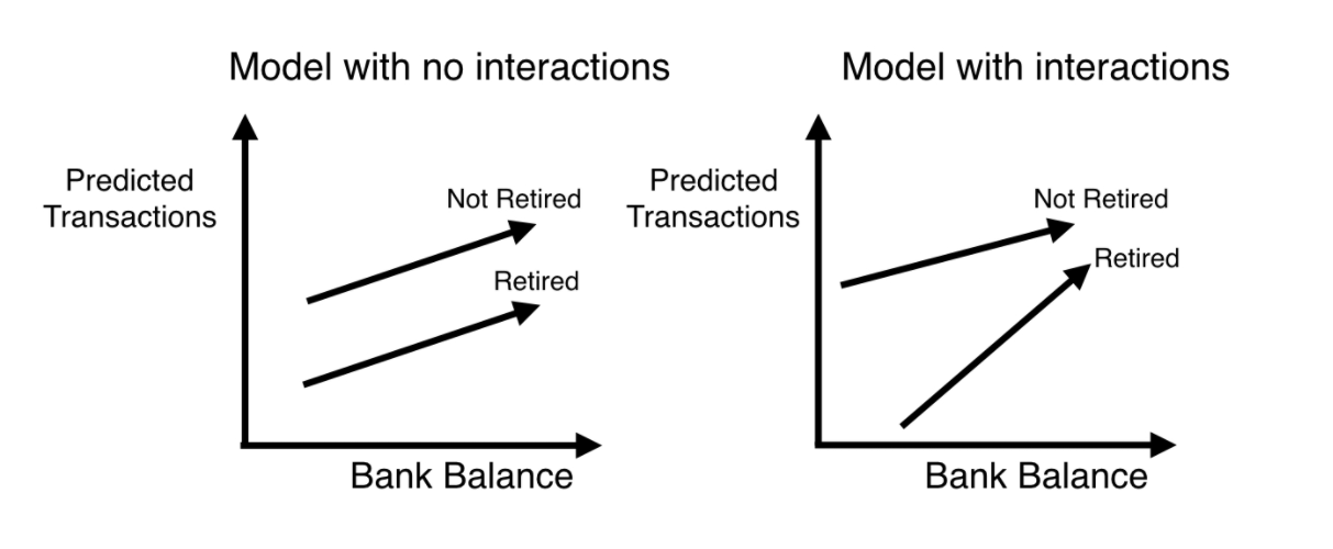
왼쪽에 있는 그림이 simple linear regression model을 도식화한 것이고 오른쪽에 있는 그림이 interaction을 고려한 model의 그림이다. 여기서 interaction을 고려한 model이 바로 deep learning의 개념이라는 것이다. 실제 현실 세계는 엄청나게 많은 요소들의 복합적 구조로 이루어진 경우가 많기에 이렇게 얽혀있는 구조의 Neural network가 바로 현실세계에서의 상호 작용을 잘 설명할 수 있는 모델링 접근 방식인 것이다. 이러한 접근 방식은 text, image, video, audio, source code 등 다양한 타입을 다룰 수 있기에 AI, DL이 기하급수적으로 관련 연구들이 쏟아지고 있는 실황이다.

---

The diagram of the neural network

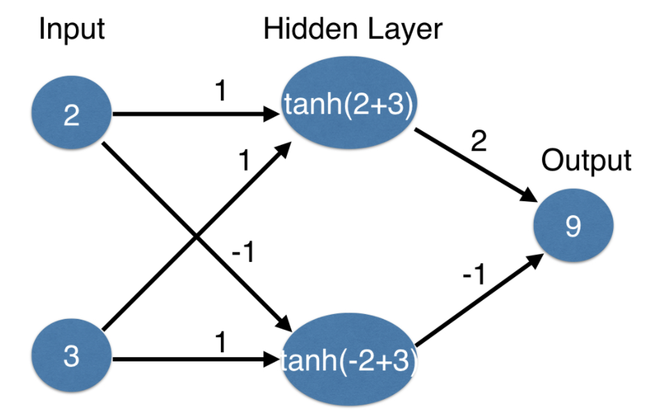
Neural network의 경우 간단한 다이어그램은 위의 그림과 같다. 가장 왼쪽은 input layer, 가장 오른쪽은 output layer이라고 부르며 input, output layer가 아닌 층을 hidden layer라고 부른다. input layer는 주어진 현실세계에서 관찰할 수 있는 요인들에 해당하며 output layer에 있는 값은 우리가 예측해야 할 값이다. Hidden layer는 우리가 data를 가지고 있거나 직접 관찰해서 얻을 수 있는 information이 아니기에 각각의 dot에 해당하는 node의 수가 많아지면 많아질수록 model이 capture 할 수 있는 interaction들이 점점 늘어나게 되는 것이다.

---

그렇다면 Neural network는 데이터를 바탕으로 어떻게 예측을 할 수 있을까?

가장 대표적인 방법으로는 Forward propagation(순방향 전파)이 있다. 

 

Forward propagation

Forward propagation algorithm은 hidden layer를 통과하면서 output layer를 예측하게 되어 순방향으로 나아가는 방식이다. 우선 input에 있는 node들이 hidden layer에 있는 node들과 각각의 line으로 connect 하게 된다. 이때 각각의 line에는 weight(가중치)를 갖게 되는데 여기서 가중치는 한 line이 끝나는 hidden node에 input node가 얼마나 영향을 미치는지를 의미한다. 예를 들어보면 hidden layer의 2개의 node 중 bottom node는 input top node의 -1의 영향을 미치고 input bottom node는 1의 영향을 미치는 것이다. 이러한 weights들은 우리가 훈련과정에서 얻을 수 있는 값이기도 하고 조정을 통해 바꿀 수 있는 값이다.

 

최종적으로 hidden layer 속 각각의 node 값을 예측하기 위해선 input layer에 해당 node에서 끝나는 weight를 곱한 다음 모든 값을 sum 하는 방식을 취한다. 예를 들면 hidden layer의 top node의 5라는 값은

hidden layer top node =( input top node(2) * weight(1) ) + ( input bottom node(3) * weight(1) )

이렇게 산출된다. 동일한 방식으로 hidden bottom node 또한 산출한 다음 output node의 값은 설정한 weight과 곱셈 후 더해 9라는 값을 얻게 된다. 이렇게 곱하고 더하는 multiply- add process는 벡터 대수나 선형 대수에서 배울 수 있는 내적의 연산과 동일한 process이다.

 

# Forward propagation using numpy
import numpy as np

input_data = np.array([2,3])
weights = {'node_0' : np.array([1,1]),
	   'node_1' : np.array([-1,1]),
	   'output' : np.array([2,-1])
            }
            
node_0_value = (input_data * weights['node_0']).sum()
node_1_value = (input_data * weights['node_1']).sum()

hidden_layer_values = np.array([node_0_value, node_1_value])

output = (hidden_layer_values * weights['output']).sum()

위의 code는 numpy를 사용하여 simple하게 forward propagation을 구현해본 결과이다.

---

 

Graphs according to linearity and non-linearity

이렇게 현실 세계에 다양하게 존재하는 요소들이 모두 선형성을 띈다면 좋겠지만 현실은 그렇지 않다. multiply-add process 즉, 내적에 의한 연산으로 hidden layer 내의 node 값들을 예측하는 것은 가장 단순하고 쉬운 구조에서만 가능한 방식이기에 비선형성을 띈 요소들을 반영할 수 있는 다른 process가 요구 시 된다.

 

 

Diagram applied tanh activation function

현실세계에서 비선형성을 반영하고 강력한 predictive model을 만들어내기 위해 생긴 개념이 바로 Activation function(활성함수)이다. Activation function을 사용하면 model이 non-linearity를 capture 할 수 있다. Activation function은 node로 들어오는 값에 적용되며 그런 다음 해당 node에 저장된 값 또는 node 출력으로 변환해준다. 오랫동안 사용돼 왔던 activation function으로는 tanh라는 S자형 함수였다. tanh는 내적에 의한 연산 후 tanh(값)을 출력하는 방식이다. 위의 예시를 그대로 적용해보자. Hidden layer의 top node는 위의 예에서 내적에 의해 5라는 값을 얻을 수 있었다. 여기서 activation function으로 tanh를 적용하게 되면 top node는 tanh(5)로 출력이 되는 것이다.

 

밑의 코드는 내적에 의한 덧셈 후 tanh activation function을 적용해 neural network를 구현해본 결과이다.

# Neural network using numpy and tanh activation function
import numpy as np

input_data = np.array([-1,2])
weights = {'node_0' : np.array([3,3]),
	   'node_1' : np.array([1,5]),
       'node_2' : np.array([2,-1])}

node_0_input = (input_data * weights['node_0']).sum()
node_0_output = np.tanh(node_0_input)
node_1_input = (input_data * weights['node_1']).sum()
node_1_output = np.tanh(node_1_input)

hidden_layer_outputs = np.array([node_0_output, node_1_output])
output = (hidden_layer_outputs * weights['output']).sum()

 

---

tanh는 오랫동안 사용되어온 강력한 activation function이었으나 오늘날 산업 및 연구 응용 분야의 표준은 ReLU(Rectified Linear Unit)이다. ReLU는 두 개의 선형 조각으로만 구성된 activation function이지만 놀라울 정도로 강력한 activation function이다. input이 negative인 경우 0을 반환하고 0을 포함하여 positive인 경우 해당 입력값을 반환하는 것이 ReLU의 구조이다. 

ReLU(Rectified Linear Unit, Rectified Linear Activation)

# Applying the network to many observations/rows of data using relu

def relu(input):
    output = max(input, 0)
    return(output)

def predict_with_network(input_data_row, weights):

    node_0_input = (input_data_row * weights['node_0']).sum()
    node_0_output = relu(node_0_input)

    node_1_input = (input_data_row * weights['node_1']).sum()
    node_1_output = relu(node_1_input)

    hidden_layer_outputs = np.array([node_0_output, node_1_output])
    
    input_to_final_layer = (hidden_layer_outputs * weights['output']).sum()
    model_output = relu(input_to_final_layer)
    
    return(model_output)

# Create empty list to store prediction results
results = []
for input_data_row in input_data:
    # Append prediction to results
    results.append(predict_with_network(input_data_row, weights))

print(results)

위의 코드는 relu function을 함수로 선언하여 이를 activation function으로 사용하되 복수 개의 데이터로 구성된 데이터에 적용하기 위하여 for문을 통해 output을 반환하는 구조를 구현해보았다. input_data가 2차원 array구조인 줄 모르고 약 3분 동안 벙쪘다..

---

Multiple hidden layers calculating with ReLU activation function

이렇게 현실세계에서의 비선형성을 반영하기 위해 activation function을 사용해야 함을 알았으니 쉽게 유추해볼 수 있는 것은 hidden layer가 과연 1개처럼 적게 이루어져 있을까이다. 물론 아니다. Hidden layer의 수는 5개, 15개도 있을뿐더러 최근 1000개의 hidden layer를 포함한 neural network 또한 쉽게 찾아볼 수 있다. 그렇다고 Hidden layer의 수에 따라 다른 방식으로 node의 값이 결정되는 것이 아니라 동일하게 forward propagation 방식으로 진행된다. 

# Multi-layer neural networks 
def predict_with_network(input_data):
    node_0_0_input = (input_data * weights['node_0_0']).sum()
    node_0_0_output = relu(node_0_0_input)

    node_0_1_input = (input_data * weights['node_0_1']).sum()
    node_0_1_output = relu(node_0_1_input)

    hidden_0_outputs = np.array([node_0_0_output, node_0_1_output])
    
    node_1_0_input = (hidden_0_outputs * weights['node_1_0']).sum()
    node_1_0_output = relu(node_1_0_input)

    node_1_1_input = (hidden_0_outputs * weights['node_1_1']).sum()
    node_1_1_output = relu(node_1_1_input)

    hidden_1_outputs = np.array([node_1_0_output, node_1_1_output])

    model_output = (hidden_1_outputs * weights['output']).sum()
    
    return(model_output)

output = predict_with_network(input_data)
print(output)

위의 코드는 multi-layer를 가진 neural network를 구현해본 결과이다.

---

Representation learning in Image Classification 

숫자 말고 image의 경우는 어떨까? 위의 예를 보면 Image Classification에서 deep network가 어떻게 진행되는지 개념을 설명한 그림이다. Deep network가 Image classification을 할 때는 먼저 한 pixel을 기준으로 근처에 있는 pixel들을 그룹으로 묶어 아주 간단한 pattern을 찾는 것부터 시작한다. 찾을 수 있는 간단한 pattern으로는 diagonal lines, horizontal lines, vertical lines, blurry areas 등을 찾을 수 있다. line들이 어디에 위치해있는지 식별한 후로는 다음 layer에서 그보다 더 큰 pattern을 발견하기 위해 찾은 line들의 정보를 합쳐서 더 큰 정보를 얻는다. 첫 번째 layer에서 발견한 vertical lines과 horizontal lines들에 대한 정보가 두 번째 layer에서는 vertical lines들과 horizontal lines들로 이루어진 정사각형에 대한 정보를 얻게 되는 것이다. 이렇게 계속 진행하게 되면 얻었던 정사각형 pattern이 곧 checkerboard pattern이었음을 식별하게 되는 방식이다. 

 

이렇게 deep network는 데이터 속 패턴을 표현하기 위해 내부적으로 설계하기 때문에 별도의 feature engineering 작업이 필요되지 않는다. Raw data를 model이 잘 이해하기 쉽게 자체적으로 표현하는 과정의 반복이기에 직접적으로 modeler가 data 속 interaction들을 따로 명시할 필요가 없다는 특징이 존재한다. Weight들 또한 model이 pattern을 표현하기 위해 스스로 학습하고 얻는 과정이기에 weight들도 명시할 필요가 없는데 이건 다음장에서 더욱 자세히 알아보기로 한다!

 

그림 출처 : DataCamp